Who are the dumpers? The Token-as-a-Product paradigm

27 March 2025 · Tarek Awwad

Why Should Anyone Buy and Hold Your Token?

In the blockchain landscape, tokens are often viewed solely through a technical lens. However, to truly thrive, a token must be treated as a product - one that people need, want, buy, use, and hold onto. In this article, I argue for the importance of this product-centric approach, specifically focusing on understanding and managing churn.

While traditional product metrics and tools are well-established, the unique context of blockchain requires innovative methods. We will explore less conventional techniques for analyzing churn to gain deeper insights into user behavior and enhance the value and appeal of tokens.

The Dilemma Shift

In the early days of blockchain, when ICOs were all the rage, founding teams and token issuers often faced a crucial question: Should they build their own blockchain, or simply launch a token on an existing one like Ethereum? This question arose due to the complexity of building a blockchain from scratch at the time - frameworks like Cosmos SDK and Substrate either didn’t exist or weren’t mature enough. Investors were particularly concerned about the feasibility and cost of developing a secure, maintainable chain client and launching a blockchain.

While launching a blockchain was a significant challenge, the speed and ease with which one could raise tens of millions through token sales in those early days made launching a token - rather than an entire blockchain - a no-brainer. This was true even when the token didn’t meaningfully contribute to the project’s value proposition. Loose or nonexistent regulations enabled market manipulation through simple market-making strategies, risky centralized exchange (CEX) tactics, and undisclosed advertising. Combined with an immature market characterized by widespread “degen” behavior, a lack of common sense, and poor risk management, these factors allowed many projects to sustain their token’s value long enough to maintain traction and survive the next bear market.

Today, we are moving toward a more rational and mature crypto market, despite some exceptions (e.g., the Trump family tokens). Institutional players, state reserves, and traditional finance firms are increasingly participating, bringing a level of rationalization by steering the market toward traditional financial and economic guidelines. This shift deprives blockchain startups and teams of the privilege of fast and easy fundraising through token launches. As a result, they now face a new era’s dilemma: should they launch a token at all?

Unfortunately, despite the market’s maturation, the temptation to launch a token often outweighs the arguments against it. The belief in succeeding where many others have failed - because “the token has real utility”, “has organic traction”, or “features novel, unbeatable tokenomics” - leads many Web3 projects, including those already successful, to launch a token anyway…

The Perspective Shift

While decentralization is the promise of every blockchain, very few blockchains are truly decentralized - whether technically (e.g., the geographical and server provider distribution of nodes), technologically (e.g., the number of clients in use), or economically (e.g., the native staking token supply). The same applies to tokens issued non-natively on third-party chains via smart contracts or token factories. Supplies are usually skewed toward the issuer, despite the illusion of decentralization created by allocations like team allocations, community pools, strategic reserves, and so on. These are typically controlled directly by the team or remain highly dependent on the team’s decisions regarding their use.

This centralization puts the responsibility of maintaining the token on the shoulder of the teams. Maintaining the token is not (only) about technically maintaining the smart contract or the blockchain that holds it. It is about making it desirable and attractive so that it holds its perceived value. In other words, the token should be treated as a product. People must need it, want it, buy it, use it, keep it and sell it only for those who see it more valuable. Very few teams treat their token as a product though.

On A Quest To Understand

A common approach for issuing and maintaining a token in the crypto space is to copy existing supposed “battle-tested” tokenomics and rely on market making (MM) as a powerful tool to control the token’s value in the market. However, MM is merely a symptomatic treatment when a token isn’t well-designed to serve its utility, when its fundamentals are weak or when its distribution doesn’t follow a strategically designed and thought-out model. Moreover, MM is a tool of privilege, as smaller projects often lack the necessary resources - liquidity and financial attractiveness - to leverage it effectively. By seeing the token as a product, teams can unlock both, a new mindset that allows them to understand an essential part of why a token is performing the way it is and the tools to address problems they identify.

On this quest to understand, I will focus in this work on an important aspect of a product lifecycle, that is churn. Churn is a key metric for measuring user retention after acquisition and onboarding. Understanding churn is essential for closing the feedback loop, enabling continuous improvement of both the product and its distribution strategies. In blockchain, assuming we adopted the token-as-a-product paradigm, churn can be defined as follows: for a token holder, it is the act of disengaging from the ecosystem, whether by selling their tokens, ceasing to participate in governance, or reducing their on-chain activity over time.

Product people have well-established metrics, tools, and processes for measuring churn. My goal is not to reinvent the wheel but to explore less conventional approaches to understanding churn within the specific context of blockchain. In the following sections, I will dive into two techniques: subgroup discovery and behavioral timeline mining.

Subgroup Discovery

A Quick Introduction

Subgroup discovery (SD) is a data mining technique that aims at identifying, in a given dataset, interesting subgroups that exhibit unusual statistical properties. It is formally defined in [1][2] as follows :

As simple as it might sound as a concept, SD is a tricky technique. Its effectiveness depends on several key factors:

1. SD is not a one-size-fits-all approach. The results it produces are highly specific to the dataset. While this limits generalization, it makes SD particularly valuable for uncovering context-specific insights.
2. Feature engineering plays a crucial role. From selection and encoding to cleaning, every step impacts an SD algorithm’s ability to navigate the search space and identify significant subgroups. The same applies to the target property, which must be carefully computed and structured to align with the search algorithm.
3. The choice of quality measure is critical. During its search, an SD algorithm relies on a metric to determine whether a subgroup is meaningful with respect to the target property. Selecting the right quality measure is essential for producing reliable inferences. Generally, the used quality measure is a derivation of the Klösgen function [3]. This measure takes into account both the size of the discovered subgroup and its statistical deviation from the overall population.
4. The search algorithm itself matters. The method used to explore the search space directly affects the quality and efficiency of the discovered subgroups. Many algorithms exist, they are either heuristic which encompasses beam search methods like CN2-SD [4] and PRIM [5] and genetic algorithms like in [6] or exhaustive like SD-MAP [7].

SD To Investigate Churn In Blockchain

Back to our blockchain context and as I mentioned earlier, fixing a token requires understanding why people are dumping it. A key part of understanding the why is identifying the who. To explore this, we can leverage subgroup discovery to answer the question: Who is dumping the token?

In this context, our population consists of token holders represented by their wallets on the blockchain. These wallets can be characterized by various attributes, such as balance, number of transactions, network connections, and type (vesting, multisig, etc.). The target property is whether a wallet belongs to a dumper. This can be framed as either: A binary observation e.g., The wallet either dumped tokens or did not. A numerical observation e.g., The amount of tokens sold.

To test this approach, I will use data from a public, permissionless Cosmos-SDK chain. The chain is relatively large but not overwhelmingly so - it has a reasonable number of active accounts and transactions. However, its token is only tradable on a single DEX (Osmosis), which simplifies tracking token flows and identifying sellers, as all selling activity occurs on one publicly searchable platform. For simplicity, let’s assume a wallet-holder parity, meaning each wallet represents a single holder.

The dataset was built by sourcing data from multiple sources: the chain RPCs for data like the balances, creation height and connections, and Osmosis RPCs and public APIs (Imperator API - now deprecated) for trading data. After some (a lot of) cleaning, labelling, balancing and merging, I ended up with a single CSV file containing ap. 15K rows-each representing a wallet- and 27 features describing these wallets.

raw_df = pd.read_csv("data/wallets_data.csv")
print(raw_df.shape)
print(raw_df.columns

(15085, 27)
Index(['address', 'account_type', 'account_number', 'sequence', 'is_mutlisig',
       'owner_type', 'number_of_connections', 'total_buy', 'number_of_buys',
       'total_sell', 'number_of_sells', 'total_swap', 'number_of_swaps',
       'average_swap_size', 'is_osmosis_neighbour', 'available_balance',
       'delegated_balance', 'undelegated_balance', 'timestamp', 'total', 
       'active', 'tenure', 'is_genesis', 'is_IC1', 'is_IC1_neighbour', 'is_IC2',
       'is_IC2_neighbour'],
      dtype='object')

Before applying our discovery algorithm we need to perform 2 steps:

• Remove unneeded features: This step is crucial for reducing noise and improving the algorithm’s effectiveness. Feature selection can be guided by domain expertise, ensuring that only meaningful and independent variables are retained.
• Define our target variables: In the example below, we use two target variables. One numerical, stt or sell-to-total ratio, and one binary called dumped. The binary variable is derived from both stb (sell-to-buy ratio) and stt, with thresholds set at 1 for the former and 0.5 for the latter. A wallet is classified as a “dumper” if it has sold more than it bought or has liquidated more than half of its historical holdings.

Let’s load our data, compute our targets and select our features:

import pandas as pd
import numpy as np
import matplotlib.pyplot as plt

raw_df = pd.read_csv("data/wallets_data.csv")

# Compute numeric targets 
# Sell to buy ratio
raw_df["dumped_stb"] = np.where(
    raw_df["total_buy"] > 0, 
    raw_df["total_sell"] / raw_df["total_buy"],
    raw_df["total_sell"] * 10  
    )

# Sell to total ratio
raw_df["dumped_stt"] = np.where(
    raw_df["total"]> 0, 
    raw_df["total_sell"] / raw_df["total"],
    0  
    )

# Binary targets
raw_df["dumped"] = (raw_df["dumped_stb"] > 1) | (raw_df["dumped_stt"] > 0.5)

# Feature selection
dimensions = [
    "sequence", # reflects the number of transactions on the chain
    "total", # total holding over time
    "active", # frequent trader
    "tenure", # months since joining
    "is_mutlisig", 
    "is_genesis",
    "is_IC1", # part of investment community IC1
    "is_IC1_neighbour", # has a connection that is part of IC1
    "is_IC2", # part of investment community IC2
    "is_IC2_neighbour", # has a connection that is part of IC2
]

df = raw_df[dimensions + ["dumped", "dumped_stb", "dumped_stt"]]
df = df[(df["total"] > 100)]  # removing very small wallet, 100 $Tokens = 50$ at avg price

print(df.shape)

(4596, 13)

Now that we have the data set up, we can apply our search algorithm (Beam search in this example). We will try both binary and numerical targets with Wracc and median quality measures respectively. I am using the pysubgroup python library which implements a wide range of search algorithms and quality measures.

import pysubgroup as ps
import pandas as pd

binary_target_feature = "dumped"
numeric_target_features = ["dumped_stt", "dumped_stb"]

# Binary target
data = df.copy()
target = ps.BinaryTarget(binary_target_feature, True)
search_space = ps.create_selectors(data, ignore=[binary_target_feature] + numeric_target_features)

task = ps.SubgroupDiscoveryTask(data, target, search_space, result_set_size=10, depth=3, qf=ps.WRAccQF())
result = ps.BeamSearch().execute(task)

r = result.to_dataframe()
r.to_csv('output/subgroups_binary.csv', index=False)

# Numerical target
data = df.copy()
target = ps.NumericTarget(numeric_target_features[0]) # using stt 
search_space = ps.create_selectors(data, ignore=numeric_target_features + [binary_target_feature])
task = ps.SubgroupDiscoveryTask(data, target, search_space, result_set_size=10, depth=3, qf=ps.StandardQFNumeric(1, centroid="median"))	

result = ps.BeamSearch().execute(task)
result.to_dataframe().to_csv('output/subgroups_umerical.csv')

The results look something like this for the binary target:

sg_id,quality,subgroup,size_sg,size_dataset,positives_sg,positives_dataset,size_complement,relative_size_sg,relative_size_complement,coverage_sg,coverage_complement,target_share_sg,target_share_complement,target_share_dataset,lift
0,0.04322052001953124,is_IC1==False,3456,4096,1295,1325,640,0.84375,0.15625,0.9773584905660377,0.022641509433962263,0.37471064814814814,0.046875,0.323486328125,1.1583508036338224
1,0.03319728374481201,is_IC1==False AND total: [1043.65:4531.29[,810,4096,398,1325,3286,0.19775390625,0.80224609375,0.300377358490566,0.699622641509434,0.49135802469135803,0.28210590383444917,0.323486328125,1.518945259725134
2,0.03248649835586548,total: [1043.65:4531.29[,819,4096,398,1325,3277,0.199951171875,0.800048828125,0.300377358490566,0.699622641509434,0.48595848595848595,0.2828806835520293,0.323486328125,1.5022535535743082
3,0.030539870262145993,is_IC1==False AND tenure: [26:32[,754,4096,369,1325,3342,0.18408203125,0.81591796875,0.27849056603773586,0.7215094339622642,0.48938992042440316,0.28605625374027527,0.323486328125,1.5128612181572494
4,0.027244865894317623,tenure: [26:32[,839,4096,383,1325,3257,0.204833984375,0.795166015625,0.2890566037735849,0.7109433962264151,0.4564958283671037,0.289223211544366,0.323486328125,1.4111750286729483
5,0.025952041149139408,is_IC1==False AND total: [287.20:1043.65[,809,4096,368,1325,3287,0.197509765625,0.802490234375,0.27773584905660376,0.7222641509433962,0.45488257107540175,0.29114694250076056,0.323486328125,1.4061879329244118
6,0.025406420230865482,total: [287.20:1043.65[,819,4096,369,1325,3277,0.199951171875,0.800048828125,0.27849056603773586,0.7215094339622642,0.45054945054945056,0.2917302410741532,0.323486328125,1.3927928675098487
7,0.02406203746795654,is_IC1==False AND tenure: [23:26[,666,4096,314,1325,3430,0.16259765625,0.83740234375,0.2369811320754717,0.7630188679245283,0.47147147147147145,0.29475218658892127,0.323486328125,1.4574695450167148
8,0.019481778144836426,is_IC1==False AND tenure: [19:23[,758,4096,325,1325,3338,0.18505859375,0.81494140625,0.24528301886792453,0.7547169811320755,0.4287598944591029,0.2995805871779509,0.323486328125,1.3254343605316872
9,0.01574975252151489,is_IC1==False AND tenure: [26:32[ AND total: [1043.65:4531.29[,255,4096,147,1325,3841,0.062255859375,0.937744140625,0.1109433962264151,0.8890566037735849,0.5764705882352941,0.30669096589429834,0.323486328125,1.7820554938956714

and like this for the numerical target:

sg_id,quality,subgroup,size_sg,size_dataset,mean_sg,mean_dataset,std_sg,std_dataset,median_sg,median_dataset,max_sg,max_dataset,min_sg,min_dataset,mean_lift,median_lift
0,122.81087920158157,is_IC1==False AND tenure: [26:32[ AND total: [287.20:1043.65[,138,4096,0.5266912934020744,0.2660998468292418,0.4835373664649707,0.42570523179710507,0.8899339072578375,0.0,1.0,1.0,0.0,0.0,1.9792994985827859,inf
1,117.85124968222611,tenure: [26:32[ AND total: [287.20:1043.65[,140,4096,0.5193575852834792,0.2660998468292418,0.48392168880310305,0.42570523179710507,0.8417946405873293,0.0,1.0,1.0,0.0,0.0,1.9517395123370915,inf
2,95.05249338488724,is_IC1==False AND tenure: [26:32[ AND total: [1043.65:4531.29[,255,4096,0.495627363874077,0.2660998468292418,0.48029651875822293,0.42570523179710507,0.3727548760191657,0.0,1.0,1.0,0.0,0.0,1.8625616278243282,inf
3,68.89361123365615,tenure: [26:32[ AND total: [1043.65:4531.29[,258,4096,0.48986425499182024,0.2660998468292418,0.4804430311740079,0.42570523179710507,0.267029500905644,0.0,1.0,1.0,0.0,0.0,1.8409039344775333,inf
4,64.8082196389683,is_IC1==False AND tenure: [19:23[ AND total: [1043.65:4531.29[,156,4096,0.49559040046119135,0.2660998468292418,0.4856420986887462,0.42570523179710507,0.41543730537800194,0.0,1.0,1.0,0.0,0.0,1.8624227197665968,inf
5,48.45943486211188,tenure: [19:23[ AND total: [1043.65:4531.29[,157,4096,0.49243377370666147,0.2660998468292418,0.48569585081970723,0.42570523179710507,0.30865882077778267,0.0,1.0,1.0,0.0,0.0,1.850560154672542,inf
6,43.97702131539977,tenure<19 AND total: [1043.65:4531.29[,73,4096,0.4950013056727126,0.2660998468292418,0.4825168657184302,0.42570523179710507,0.6024249495260242,0.0,1.0,1.0,0.0,0.0,1.8602089086896714,inf
7,43.97702131539977,is_IC1==False AND tenure<19 AND total: [1043.65:4531.29[,73,4096,0.4950013056727126,0.2660998468292418,0.4825168657184302,0.42570523179710507,0.6024249495260242,0.0,1.0,1.0,0.0,0.0,1.8602089086896714,inf
8,36.7240420501258,is_IC1==False AND tenure: [23:26[ AND total: [287.20:1043.65[,198,4096,0.4602186107251902,0.2660998468292418,0.4734010164413556,0.42570523179710507,0.1854749598491202,0.0,1.0,1.0,0.0,0.0,1.7294959625456523,inf
9,33.907314294561296,is_IC1==False AND tenure: [23:26[,666,4096,0.42460393369280736,0.2660998468292418,0.47113708108640184,0.42570523179710507,0.050911883325167114,0.0,1.0,1.0,0.0,0.0,1.5956564378080185,inf

The results suggest several key insights about token holder behavior:

• Investment Community (IC1) as Strong Holders

  Members of the Investment Community (IC1) appear to be more committed holders. The subgroup is_IC1==False is overrepresented among sellers, indicating that retail participants are the primary drivers of churn, rather than institutional or long-term committed wallets.

• Tenure & Market Cycles

  Holders who joined between two to two and a half years ago (tenure: [26:32[) exhibit higher-than-average selling activity. This pattern may correlate with the natural lifecycle of unsuccessful Web3 projects - where early believers gradually lose confidence - or with broader bear/bull market cycles, as some holders exit positions based on macroeconomic conditions rather than project fundamentals.

• Small Holders Have Weaker Hands

  Wallets with smaller holdings (total: [1043.65:4531.29[) tend to sell more than the average. This suggests that small-scale investors are more prone to panic selling or quick profit-taking, whereas larger holders may have stronger conviction or strategic incentives to remain engaged.

Beyond This Proof of Concept

While writing this sample script, I uncovered numerous intriguing patterns worth further exploration. This test is purely illustrative and does not fully demonstrate the depth of insights SD can extract from the data. Nor does it show all the steps of a scientifically rigorous workflow that ensures the data is not skewed in a way that compromises the validity of the final result.

Moreover, addressing some of the simplifications made for the sake of clarity in this article could lead to straightforward improvements. For instance, while I am using individual wallets as our observation, one can leverage the connection graph between the wallets to identify, albeit roughly, real individual holders. Moreover, the behavior of an individual wallet can be studied to infer specific wallet groups such as market makers, team wallets, community wallets and other unlabeled wallets.

Mining The Behavioral Timeline

In the previous section, I addressed one facet of churn: token selling. Dumping the token directly impacts its price, making it a key area of interest when studying churn. However, it is not the only relevant aspect. As defined earlier, reducing on-chain activity and decreasing governance participation are also important indicators of churn. These aspects are particularly valuable because, when analyzed correctly, they can help predict future token dumps.

What Is A Behavioral Timeline

While computing basic statistics - such as the trend of governance-related transactions, the number and amount of staking transactions per epoch, and ongoing undelegations or unstaking events - can quantify on-chain activity in a mathematically sound manner, I believe data visualization offers a more effective way to investigate and navigate such activity.

In this section, I will introduce a visualization technique I call the Behavioral Timeline. It is a simple yet effective technique that consists of doing the following:

• For each transaction type assign a specific color.
• Create a one dimensional axis that represent the timeline. The x values are the block heights. Restrict the width of the timeline (don’t make it scale w.r.t the number of data points) since the density matters as we will explain later.
• On the timeline, trace a vertical line for each transaction in the history with the corresponding color.

I implemented a version of this approach using Python and Dash. I will provide a guide on how to replicate it in a separate post and link it here in the future. The final result should look something like this:

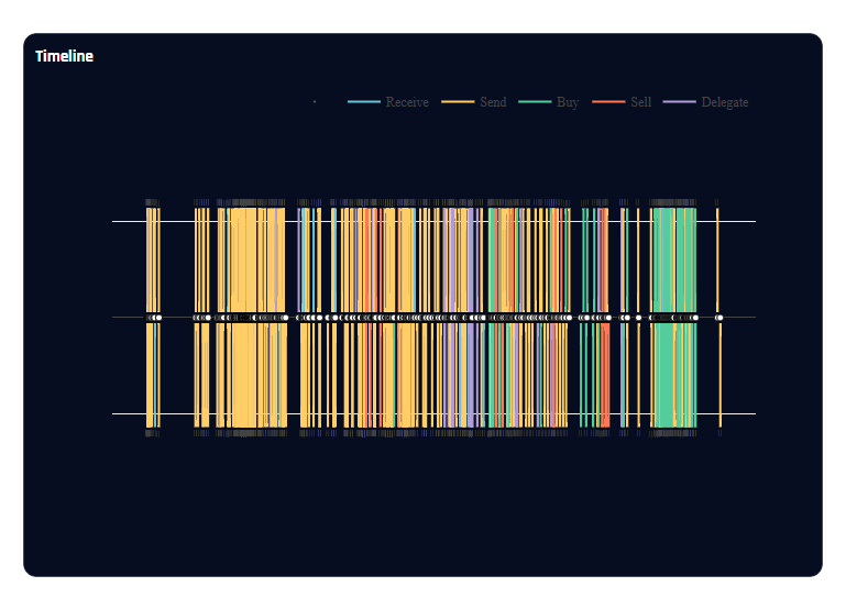
This visualization provides several key benefits:

• It clearly highlights activity types and their transitions - for example, a shift from buying and staking to unstaking i.e., shifting from commitment to disengagement.
• It reveals participation trends. A denser timeline indicates a higher participation rate, allowing for the identification of participation gaps. These gaps may reflect a holder’s mindset - such as disengagement, renewed interest - or external factors like the discovery of new financial opportunities or even malicious behavior.
• It abstracts unnecessary details - such as transaction amounts and addresses. While these details are valuable, incorporating them during the exploration phase can be overwhelming. This is particularly evident in the subgroup discovery use case discussed earlier, where the complexity of formalizing the problem increases due to the mathematical definition of dumping, which depends on transaction amounts and wallet balances.

Uncovering Churn Patterns

Here are few examples of interesting patterns that can indicate some churn aspects:

1. The defector behavior

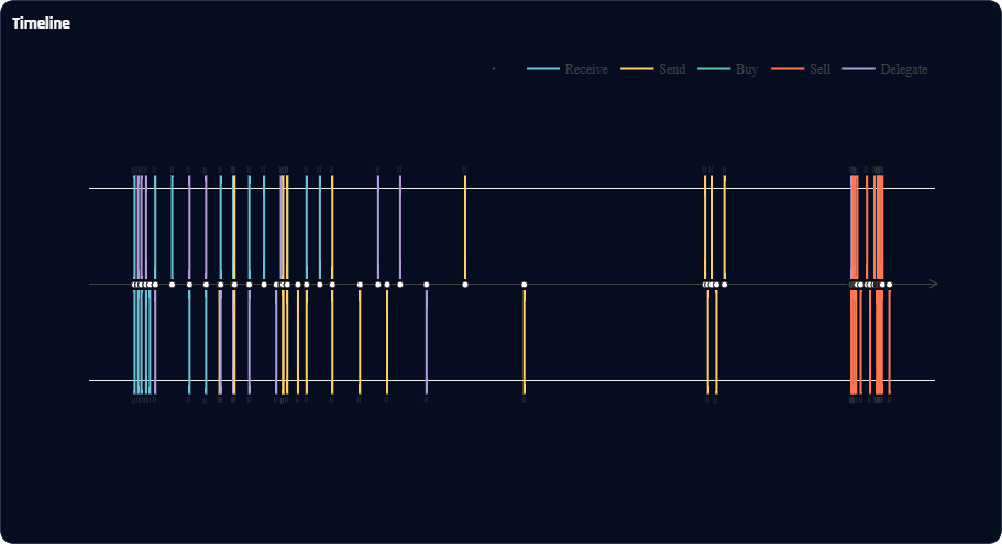
This timeline clearly illustrates a complete lifecycle. It begins with receiving tokens (onboarding) and delegating them (commitment), followed by a period of regular token usage. This is then interrupted by a significant phase of inactivity (disengagement and “soft” churn), ultimately leading to heavy selling activity, which signifies hard churn.

2. The latent defector behavior

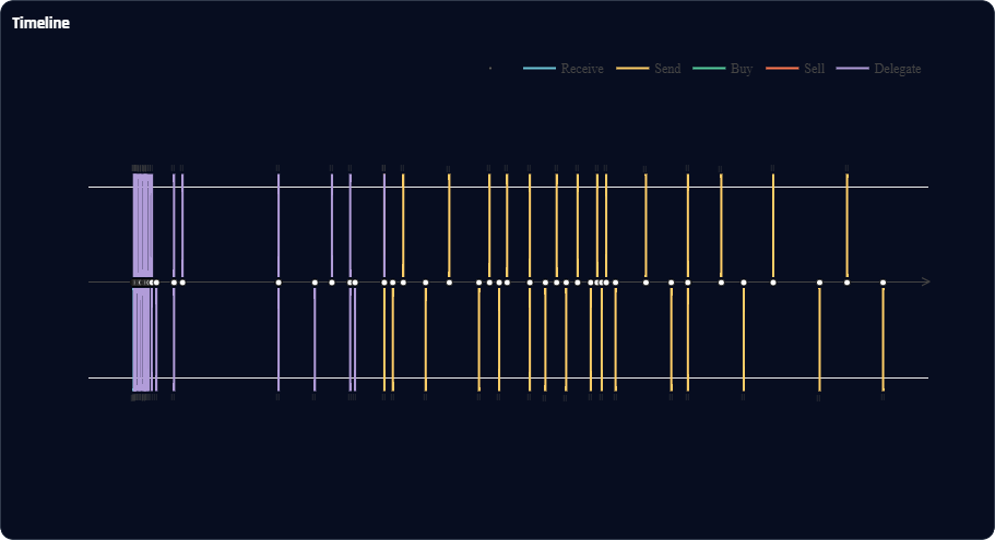
This timeline illustrates a holder in the second half of the timeline described in the previous case. The user transitioned from a strong commitment (dense delegations) to a more casual disengagement, characterized by low activity and qualitatively lower commitment transactions (sends). Based on this, one could classify this holder as a prospective dumper.

3. The salient shifter

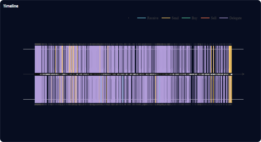
This timeline reflects a shift in the holder’s behavior without necessarily indicating a churn risk. The holder has transitioned from a long period of high-commitment transactions (dense delegations) to a shorter period of low-commitment transactions (sends). However, the transaction density remains high, which can be interpreted either positively (existing interest to be investigated) or negatively (an upcoming rage quit).

4. The skeptical believer

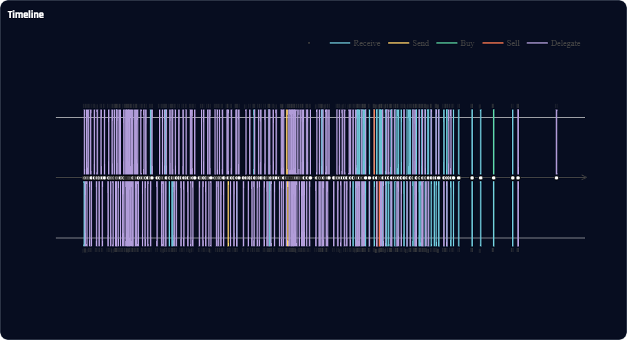
This timeline is characterized by an decreasing transaction density, which may suggest growing disengagement and emerging skepticism toward the token. However, this profile remains particularly interesting, as the type of transactions - such as delegations - reflect residual interest, given that delegation requires a relatively high level of commitment.

Here are other interesting patterns which I won’t discuss in this post:

1. The exit wallet

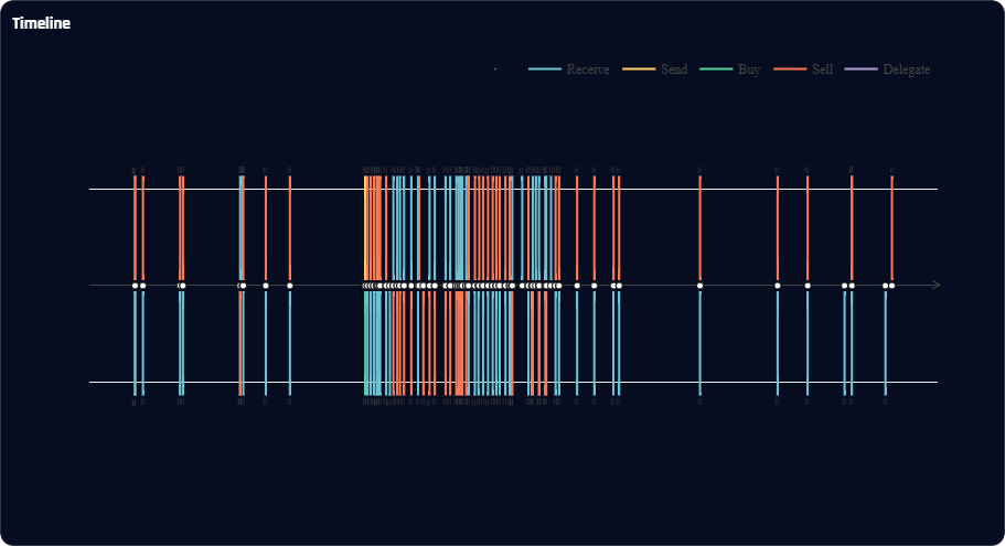
2. The profit taker

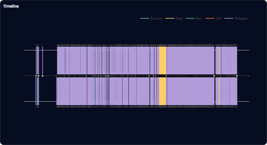
Using this technique alone is not scalable - no one could, or should, manually visualize the data for every wallet on the chain. However, it serves as a valuable preliminary or complementary step for other techniques, such as clustering and subgroup discovery (SD). For example, it can help identifying patterns which in turns can guide feature selection (e.g., identifying key behaviors to model), validate algorithmic findings (e.g., checking if clusters reflect real patterns), and reveal hidden relationships (e.g., coordinated dumps). This approach can also be enhanced with additional filters and tags, though these are topics for future discussions.

For now, here’s a sneak peek…

https://drive.google.com/file/d/1MRecnDPq-GxdxCy178GFwjmCTzh91NeB/view?usp=sharing

Some Closing Thoughts…

In this article I highlighted the importance of treating a token as a product to improve its chances of success in the rapidly evolving blockchain space. I focused on a critical aspect of a product’s lifecycle, the Churn, and explored practical approaches to better understand and analyze it. These insights and tools can help projects make informed decisions to enhance retention and long-term sustainability.

Of course, I may have overlooked something important. Readers, I’d love to hear your thoughts - what other challenges make treating a token as a product even harder than I imagined?

References

[1] W. Klösgen, Exploration of Simulation Experiments by Discovery, in Knowledge Discovery in Databases: Papers from the 1994 (AAAI) Workshop (Seattle, Washington, USA), 1994, pp. 251-262.

[2] S. Wrobel, An algorithm for multi-relational discovery of subgroups, J. Komorowski and J. Zytkow (editors), Principles of Data Mining and Knowledge Discovery, Springer, Berlin, Heidelberg, Vol. 1263, 1997, pp. 78-87. PKDD 1997

[3] W. Klosgen. Explora: A multipattern and multistrategy discovery assistant. Advances in Knowledge Discovery and Data Mining. AAAI/MIT Press, 1996

[4] N. Lavrac, B. Kavsek, P. Flach, and L. Todorovski. Subgroup Discovery with CN2-SD. Journal of Machine Learning Research, 5:153–188, 2004.

[5] J. H. Friedman and N. I. Fisher. Bump Hunting in High-Dimensional Data. Statistics and Computing, 9(2), 1999.

[6] C. J. Carmona, P. Gonzalez, M. J. del Jesus, and F. Herrera. Overview on Evolutionary Subgroup Discovery: Analysis of the Suitability and Potential of the Search Performed by Evolutionary Algorithms. Wiley Interdisciplinary Reviews: Data Mining and Knowledge Discovery, 4(2):87–103, 2014.

[7] M. Atzmueller and F. Puppe. SD-Map - A Fast Algorithm for Exhaustive Subgroup Discovery. In Proc. PKDD, volume 4213 of LNAI, pages 6–17, Heidelberg, Germany, 2006. Springer Verlag.

[8] Subgroup Discovery and its application to SQL workload Analysis by Anes Bendimerad

[9] M. Atzmueller. Subgroup discovery. Wiley Interdisciplinary Reviews: Data Mining and Knowledge Discovery 5.1, 2015.

[10] Remil, Youcef, et al. “What makes my queries slow?”: Subgroup Discovery for SQL Workload Analysis. 2021 36th IEEE/ACM International Conference on Automated Software Engineering (ASE). IEEE, 2021.

First published on the Sydyk blog, March 2025.